
Many mechanical components operate in environments subject to vibration, which is likely to cause resonance if the components have low eigenfrequencies. This can have effects of varying severity, whether it be a mild nuisance for an automotive trim, critical errors in high-precision manufacturing, or a dangerous failure in civil engineering. This blog post demonstrates how to maximize the lowest eigenfrequency using shape and topology optimization so that the likelihood of resonance can be reduced. The built-in functionality of the COMSOL Multiphysics® software allows for solving these problems with gradient-based optimization.
Introduction to Mechanical Resonance
When a mechanical system is excited by a force whose frequency content matches the natural frequencies of the system, mechanical resonance can occur, leading to vibration with a high amplitude. This effect can be taken advantage of (e.g., in watches and musical instruments), but in this blog post we will focus on unwanted resonance, which can cause fatigue problems in machines or failures in civil engineering. Several measures can be taken to mitigate resonance, such as installing active or passive vibration isolation systems or instructing users to avoid resonance-inducing behavior. For instance, as seen in the image below, a famous bridge in London includes a sign that instructs soldiers to break step when crossing the bridge — that way the unified rhythm of their marching will not cause dangerous mechanical resonance.
Another strategy for avoiding mechanical resonance is to simply increase the lowest natural frequency. Here, we’ll explore how this can be achieved with optimization.

The Albert Bridge in London includes a sign instructing soldiers to break step on the bridge to avoid resonance. Original image by Colin Smith, licensed under CC BY-SA 2.0 via Wikimedia Commons.
Introduction to Optimization
All optimization problems consist of some design variables that should be changed by an optimization algorithm in order to improve a certain quantity — the objective function. There may also be requirements where other variables cannot exceed certain bounds, also called constraints. In the context of CAD, the objective is often computed using simulation.
For the optimization algorithm, one can distinguish between:
- Gradient-free optimization, where the optimization only uses the values of the objective and constraints to update the design variables
- Gradient-based optimization, where the optimization also knows how sensitive the objective and constraints are to changes in the design variables
Gradient-based optimization has significantly more information in every iteration and is therefore significantly faster, particularly for problems with many design variables. The speed discrepancy is so large that the first approach is impractical for most applications of shape and topology optimization. COMSOL Multiphysics® supports both optimization types listed here, but this blog post will focus on gradient-based optimization.
In the following examples, the objective is to maximize the minimum eigenfrequency, but one could also maximize the distance to some unwanted frequency that is perhaps occurring naturally in the environment. A recurring aspect of eigenfrequency problems is that even though a structure contains design symmetries, its eigenmodes may be nonsymmetric. For this reason, the whole structure has to be modeled in every iteration. However, in the case where the initial design is symmetric, then this can be preserved using the Mirror Symmetry feature in the Shape Optimization or Topology Optimization interface.
Shape Optimization
The first example is a shell model that is fixed at one end. The continuity of the normal vector is preserved by using partial differential equation (PDE)-based regularization for the boundary deformation, \mathbf{d}, similar to the Helmholtz filter used for topology optimization, i.e.,
where d_\mathrm{max} is the maximum displacement, L_\mathrm{min} is a filter length, d_\mathrm{max}/L_\mathrm{min} is the maximum slope of the deformation, and \mathbf{c} is the control variable field of the boundary deformation. When performing shape optimization of solids, there is also a PDE for the smoothing of the interior elements, but in practice, everything is handled by the Free Shape Domain, Free Shape Boundary, and Free Shape Shell features in the Shape Optimization interface. These features only allow for gradient-based optimization. As alternatives to the PDE-based shape regularization, one can also use a polynomial regularization technique or make simple changes to the geometry, such as translation, rotation, and scaling. (Learn more about translation and scaling in our two-part series on shape optimization in electromagnetics.) The animation below shows the result of using the PDE-based regularization while preserving the symmetry of the design.
The design of the shell is animated throughout the optimization history.
Mode switching is handled by always solving for the first six eigenfrequencies and using the method of moving asymptotes (MMA) to maximize the minimum eigenfrequency.
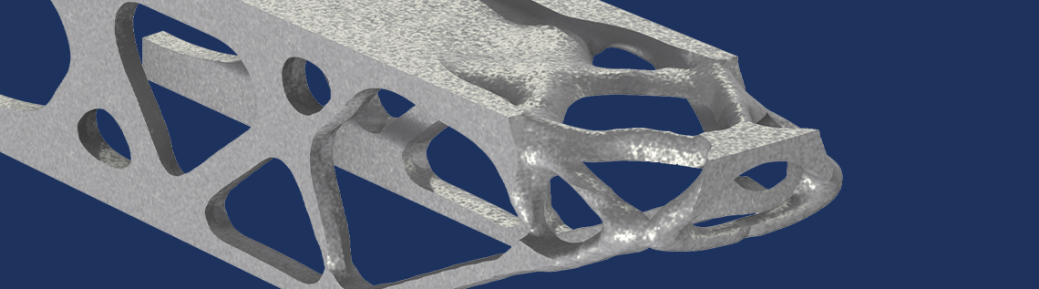
The next example considers a solid bracket, but the bracket geometry is somewhat shell-like, so it makes sense to preserve the thickness of the bracket arms. This can be achieved by combining a General Extrusion operator with a Prescribed Deformation feature (see Bracket — Eigenfrequency Shape Optimization in the Application Gallery to learn more). Otherwise, the setup is similar to the previous model in terms of the objective and enforcement of symmetry, but the initial design is not so bad, and therefore the improvement is less dramatic (as illustrated below).

The optimization history is shown with insets, illustrating the initial and optimized bracket geometry for the first and second eigenmode, respectively. The bracket is fixed at the four small holes.
Topology Optimization
Gradient-based optimization can also be taken advantage of when performing topology optimization, particularly when using the Topology Optimization interface in the software. A detailed introduction to topology optimization can be found in our blog post “Performing Topology Optimization with the Density Method”. The basic idea is to introduce a spatially varying design variable field, \theta_c, that is bounded between 0 and 1, corresponding to void and solid material, respectively. For structural mechanics, one can then let the density and the Young’s modulus (the stiffness) depend on this variable. The dependence is not explicit, as it’s advantageous to regularize the problem with a minimum length scale, L_\mathrm{min}. It’s also necessary to interpolate the density, \rho, in a different way than the stiffness, E, to prevent intermediate values of the design variable from dominating the optimized design due to their good stiffness-to-weight ratio. The relationship between the design variable field and the material properties is given by:
where \theta_f is the filtered design variable, \beta is the projection slope parameter, and p_\mathrm{SIMP} is the solid isotropic material with penalization (SIMP) parameter. These parameters can have a strong influence on the optimized design, so in order to avoid bad local minima it can be necessary to solve the optimization problem for several combinations of these two parameters. That is, a parametric sweep of optimization problems is solved, as illustrated for the beam example shown below. The beam is fixed to the left and supports a weight at the right end, which is 15% of the total weight. The beam is subjected to a 40% volume constraint. The topology optimization problem is solved for five combinations of the parameters (p_\mathrm{SIMP}, \beta), equal to (1, 2), (2, 4), (3, 8), (4, 16), and (5, 32). Poor connectivity and grayscale is expected for the initial optimizations, but these unphysical designs provide good initial designs for the later optimizations.
The design of a beam is animated throughout the optimization history. The displacement is shown via the colors on the \theta=0.5 contour.
When performing topology optimization, it’s good practice to perform a verification simulation on a body-fitted mesh. This has been done in the Application Gallery version of this model, and the results show better performance in terms of higher eigenfrequencies relative to the raw optimization result. This is to be expected, as the implicit design representation causes the material to be less stiff near the solid–void interface.
Finally, a single optimization result is shown here, but it’s easy to generate alternative designs by using different values for the volume fraction, added mass, or minimum length scale.
Conclusion
It’s possible to use shape and topology optimization to perform eigenfrequency maximization. Symmetry conditions often cannot be imposed on the physics, but one can restrict the optimization so that a symmetric design is still produced. The max/min strategy used for handling mode switching could also be applied if the objective was to maximize the distance to a certain unwanted frequency.
To gain hands-on experience with eigenfrequency maximization, download the examples mentioned in this blog post from the Application Gallery:

Comments (1)
Kayemba Augustine
February 1, 2024This is resourceful, I wonder if other structural stiffness maximizing methods such as (appropriate) mass optimization that too result into a modified/optimized geometry are superior/inferior to the Eigen Frequencies optimization method